
Last Modified on January 7, 2025
Did you know, you could easily match up vertical arrays of large data sets with just a simple formula?
VLookup in Google Sheets is a function that enables us to search for a certain value in the table array with just a simple line of code.

Subscribe & Get our FREE GA4 Course for Beginners
In this guide, we’ll understand the methods of performing Google Sheets VLookup functions on a tab and on multiple spreadsheets.
An overview of what we’ll cover:
- How to use Google Sheets VLookup from another tab?
- Using VLookup in Google Sheets from multiple tabs
- How to use Google Sheets VLookup from another sheet?
- Using VLookup in Google Sheets from multiple sheets
So let’s start!
How to use Google Sheets VLookup from Another Tab
Let’s understand how to use Google Sheets VLookup to get data from another tab.
For our reference, we’ll consider a VLookup Google Sheets example, where we have a random list of Employee IDs in the sub sheet named Sheet1.
We want to find the names of the employees corresponding to the data we have in column 1 of our sheet.

In another sub sheet named Employee Data 1, we have complete data about 15 employees including their Name, Address, and Employee ID.

Similarly, we also have an Employee Data 2 sub sheet that contains the data corresponding to 15 other employees from our organization.

And similarly, we also have an Employee Data 3 sub sheet that contains the data regarding 15 other employees from our organization.

We want to do a lookup from all the three Employee Data sub sheets to pull the data in our Sheet1.
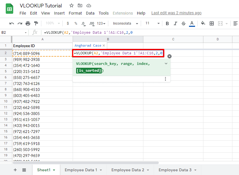
1. Let’s call the lookup function by inputting =VLOOKUP. Next, we’ll need to configure the search_key, range, index, and whether our function is sorted or not.
2. Suppose we want the function for our first Employee ID. This ID will be our search_key. As this ID is in the A2 cell, we’ll enter the same location. Add a comma after the location.
3. Next, we need to input the range. Our first data set is from the sheet named Employee Data 1. Navigate to the sheet, and select the whole range of data. Again add a comma.
4. Our next parameter is the index. This parameter signifies the column from which we want to extract the information corresponding to our search_key. As our information is the name of the employee from column 2, our index will be 2.
5. Finally, we need to mention whether our data is sorted or not. As this data is not sorted, let’s add a 0 after a comma.
6. Close the parentheses once the input is configured.
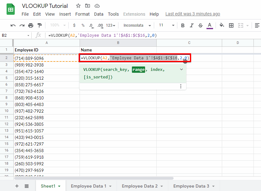
One important consideration while calling the VLookup function is the range that we configured.
7. We need to drag this formula to all the other cells in Sheet1 so it can be a generalized formula. Make the range an absolute reference by selecting the range value and clicking on F4.
8. Once done, drag this formula to cover all the employee IDs. You’ll notice that a lot of the names will be added in column B.
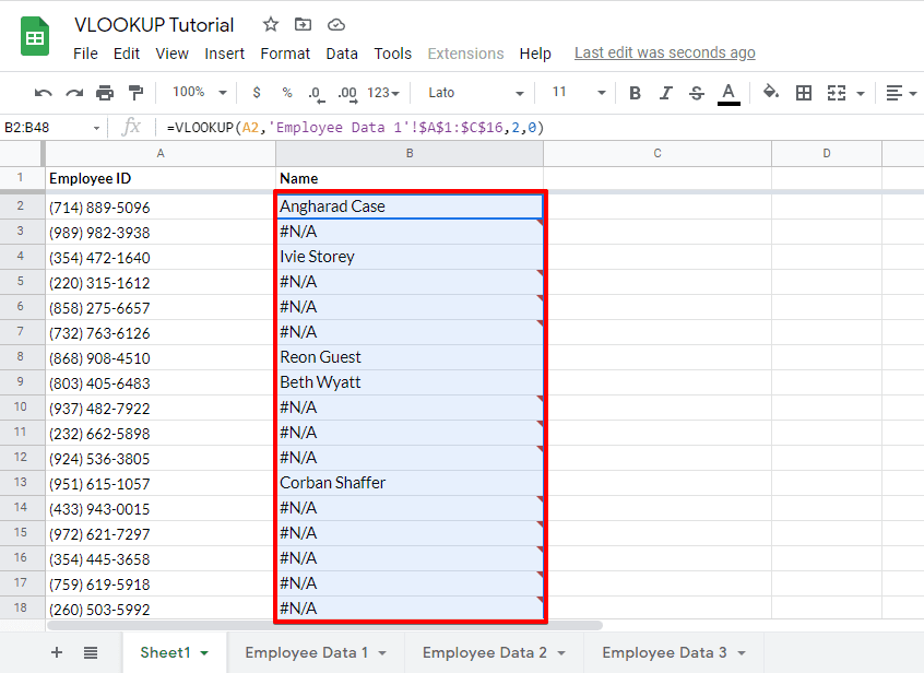
However, we still need to configure the Employee Data 2 and Employee Data 3 sheets in order to obtain all the names.
Using VLookup in Google Sheets from Multiple Tabs
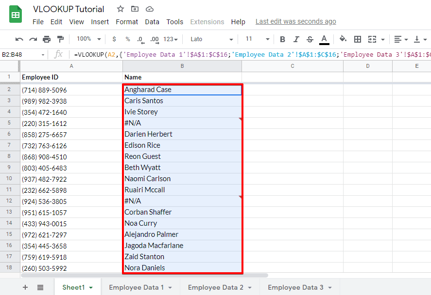
1. Let’s modify our range into an array by using curly brackets {} to denote the values.

2. We can add multiple sheets to this array now. We’ll add a semicolon after the range of the first sub-sheet ends within the curly brackets.
Following that, we’ll again add the range for the second and the third sub-sheet. The process will be the same as we added for the first sheet.
3. Make the range an absolute reference by selecting the range value and clicking on F4.

4. Drag this formula to cover all the data sets. If the formula is configured correctly, you’ll see that all the IDs have been added correctly!
🚨 Note: If the data isn’t represented correctly, it could be due to an error.
Make sure that your search key is in the same column in each sub sheet. This is because we have added a single value of the search key in our formula.
So, the order of your columns should be the same in all the sub sheets that contain the data.
However, there might be some entries that don’t show any Employee Name corresponding to the Employee ID.
This is simply because the data of those IDs don’t exist in any of our Employee Data records.
How to use Google Sheets VLookup from Another Sheet
Let’s say you have the data in different spreadsheets instead of sub sheets. The method is slightly different if you want to integrate the data for Google Sheets VLookup from another sheet.
Our current formula won’t work because our range has changed. But the essence of our new formula is similar to the one we already created.
This means we’ll still check the second column of our data to match the first column for VLookup.
Suppose we want to add Employee Data 1, Employee Data 2, and Employee Data 3 spreadsheet information into Sheet1.
1. For making it easier to understand, let’s start by adding the range values from the Employee Data 1 spreadsheet. We’ll need to import the range from various tabs into the one in which we’re collaborating the data.
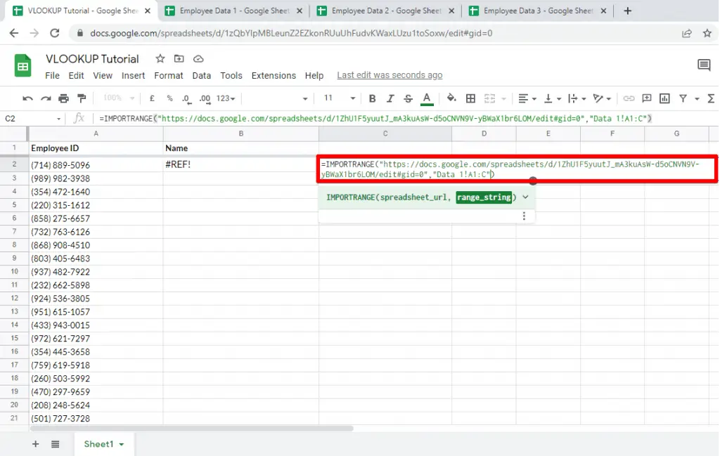
2. The import function should always be in a new cell. Call the import range function by typing =IMPORTRANGE. There will be two parts for this function – adding the sheet URL, and adding the range string.
3. The first one is to add the sheet URL. Copy the Employee Data 1 spreadsheet URL. As our URL is in a text format, we’ll add it in double-quotes “URL”. Add a comma after configuring the first parameter.
4. Next, we’ll add the range in the form of the string, so again in double-quotes. As we want the data from a sub sheet under Employee Data 1 named Data 1, we’ll keep the range as Data1!A2:C.
5. Click on Enter after filling up all the information. If the configuration is correct, you’ll be prompted to request access to Employee Data 1 sheet.

6. Once you allow access, it will establish a connection with the sheet.
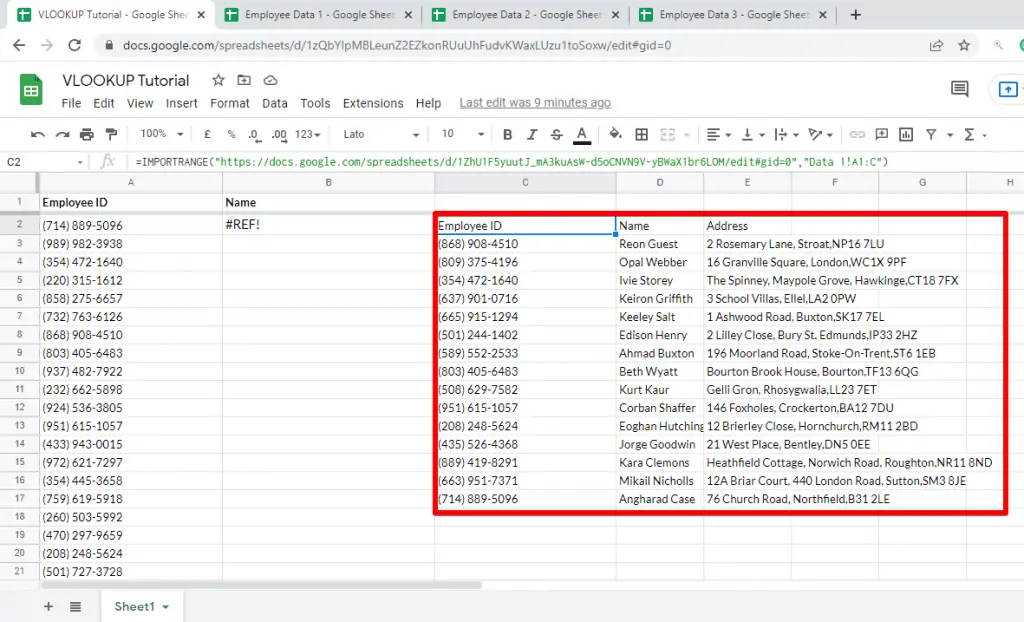
If the configuration is successful, it will show a list of the whole data set that originally appeared on the Employee Data 1 sheet.
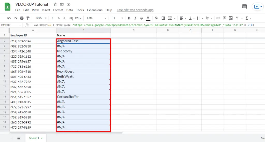
7. The range of our VLookup function will be the entire import function. Copy the whole function after the equal to sign. Paste the entire import function as the range of the VLookup function.

8. Click Enter to save the changes to the formula.
9. Once done, you can also remove all the data from the Employee Data.
10. Drag the formula to all the Employee IDs so that your data is visible.
This way, we have connected the data from another sheet to our VLookup function.
Let’s see how to connect the data from multiple sheets to do a VLookup.
Using VLookup in Google Sheets from Multiple Sheets
We’ll follow the same process for adding all three Employee Data sheets to our Sheet1.
One most important thing to remember is that we need to add each sheet individually and allow them access to the data.
The request access option is essential for configuring the data from multiple sheets to do a VLookup.
1. Just like adding the ranges of multiple tabs, we’ll add the ranges of various Employee Data sheets separated by a semi-colon.

Once you’ve added the ranges of all the sheets, your VLookup function is ready.
2. Drag your code to the entire data set for doing a VLookup.

Your configuration is successful if your data comes up correctly.
There might be some entries that don’t show any Employee Name corresponding to their Employee ID.
This is simply because the data of those IDs don’t exist in any of our Employee Data records.
FAQ
How can I use VLOOKUP in Google Sheets from another tab?
To use VLOOKUP from another tab, you need to configure the formula with the search key, range, index, and sorting options. The range should be selected from the desired tab containing the data you want to retrieve. Drag the formula across all the cells to populate the desired information.
Can I use VLOOKUP in Google Sheets from multiple tabs?
Yes, you can use VLOOKUP in Google Sheets from multiple tabs. To do this, modify the range into an array by using curly brackets {}. Add the range for each tab separated by semicolons within the curly brackets. Drag the formula across the cells to retrieve information from multiple tabs.
How can I use VLOOKUP in Google Sheets from another sheet?
If you have the data in different spreadsheets instead of sub sheets, you can use the IMPORTRANGE function to import the data into the sheet where you want to perform VLOOKUP. Use the IMPORTRANGE function to import the desired range from the other sheet and then use that imported range as the range for your VLOOKUP function.
Summary
So that’s all you need to know about performing Google Sheets VLookup functions on a sub-sheet as well as multiple spreadsheets.
These functions are especially useful when you want to match up vertical arrays of data from large volumes of data sets.
If you’re new to Google Sheets, a good idea is to start with our Google Sheets Basics guide.
Were you able to establish VLookup functions across your sheets? Which method did you use – VLookup for sub-sheets or VLookup for spreadsheets? Let us know in the comments below!

Subscribe & Get our FREE GTM for Beginners Course...


")