Google Sheets Basics – Guide for Beginners

Last Modified on January 16, 2024

Spreadsheets are essential for digital marketers, but not all marketers know how to use the basics of tools like Google Sheets to their full advantage.

In this guide, we’ll teach you how to use all the essential features of Google Sheets so that you can organize your digital marketing efforts, collaborate with teammates, and more (you can even use Google Sheets for tracking with Google Tag Manager).

Subscribe & Get our FREE GA4 Course for Beginners

GET THE FREE COURSE

An overview of what we’ll cover in this tutorial:

• How to Create a new spreadsheet in Google Drive
• Convert and import other file types into Google Sheets
• Organize individual spreadsheets in one Google Sheets file
• Navigate and organize data: columns and rows
• Creating a database
• Most useful shortcuts, navigation, and selection hotkeys
• Format data and cells
• Basic organization features in Google Sheets
• Calculations and data analysis in Google Sheets
• Use comments and notes to collaborate
• Download your spreadsheet
• Share your spreadsheet with others

So let’s dive in!

🚨 Note: Google Sheets 101, you’ll need an active Google account. Make sure your account is set up before getting started!

How to Create a New Spreadsheet in Google Drive

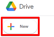
1. In Google Drive, you can create a new spreadsheet by clicking New.

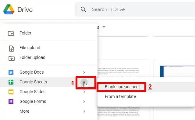
2. Hover over the arrow next to Google Sheets and select Blank spreadsheet. (You can also add a sheet with these options by right-clicking in the desired Drive location, such as inside a folder.)

If you already know that there’s a particular template you want to use, you can select one from the Google templates gallery. You can also create and upload your own templates as you get more familiar with Google Sheets.

💡 Top Tip: Love shortcuts? You can also create a new blank spreadsheet by typing sheets.new in your browser address bar.

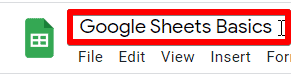
You can name the sheet in the top left corner. Just like any local file on your computer, you should give this sheet an informative name that will help you find it in your Google Drive.

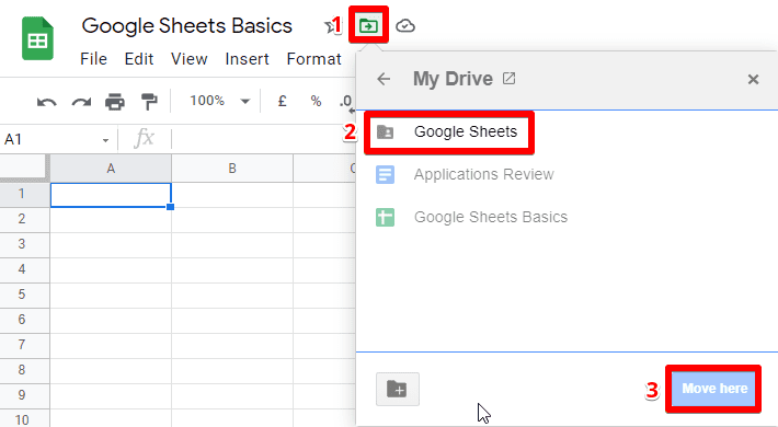
If you didn’t place this sheet in a particular Drive location yet, you can still move the spreadsheet to an existing folder or create a new folder for it.

To do this, click the small folder icon with an arrow inside and select the desired location. Then, click Move here.

Convert and Import Other File Types into Google Sheets

You can simply drag-and-drop or upload files such as Excel or CSV to Google Drive, but you would then need to make a converted copy if you wanted to edit them as a Google Sheet.

To avoid converting each file manually:

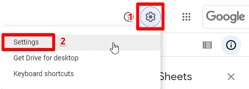
1. Click on the settings icon in your Drive and click Settings.

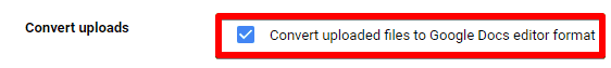
2. Then, tick the box next to Convert uploaded files to Google Docs editor format. 

Now, any file added to Google Drive will now be automatically converted to Google format without filling your Drive space with copies.

However, if you didn’t have that box checked, you can still convert your files manually. To do this, simply right-click the file and select Open with → Google Sheets.

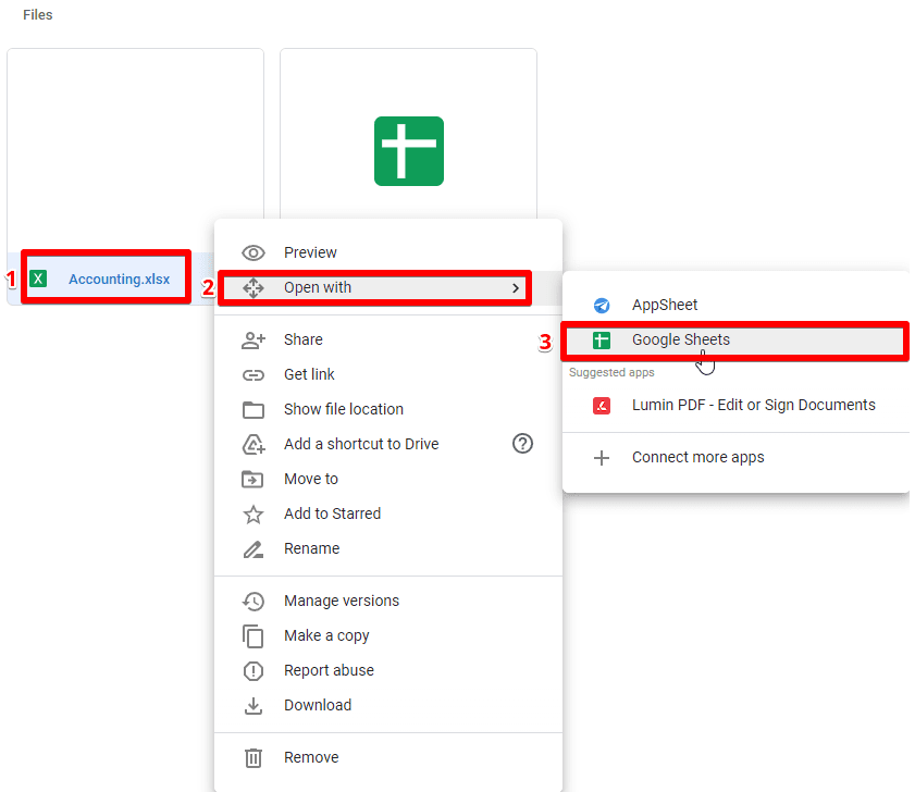
A sheet copy will be created in the same folder with the same title, but with the Google Sheets file type.

Importing Data into Google Sheets

Whether you have data in another spreadsheet, a CSV file, or even from a webpage, Google Sheets has got you covered.

Here’s how to import data into Google Sheets from different sources:

1. From Another Spreadsheet:
   • Open the Google Sheets document where you want to import the data.
   • Click on File > Import.
   • Choose the Upload tab and drag the file or click on Select a file from your device.
   • Select the file and choose how you want to import the data (replace spreadsheet, append sheets, etc.).
2. From a CSV or Excel File:
   • Follow the same steps as above. Google Sheets will automatically detect the file type and import the data accordingly.
3. From a Webpage (Web Scraping):
   • Use the IMPORTHTML function. For example, to import a table from a webpage, you’d use: =IMPORTHTML("URL", "table", index), where “URL” is the webpage’s address, and “index” is the number of the table on that page.

Tips:

• Always double-check the imported data for any inconsistencies or errors.
• For large datasets, consider using Google Sheets’ Data Connector for BigQuery.

Organize Individual Spreadsheets in One Google Sheets File

Making edits in Google Sheets is really simple, and you don’t have to worry about losing data if something unexpected happens.

All changes will be saved automatically while your computer is connected to the internet, and you can even enable offline editing that will update the Cloud file once your computer reconnects to the internet.

You’ll always know how recently your edits were saved by checking the top bar. We can see here that the last save was made recently.

If you see this message, you don’t have to worry about saving.

💡 Top Tip: You can click the “save” message to see older versions of the current document, which is useful if you need to recover something that was overwritten.

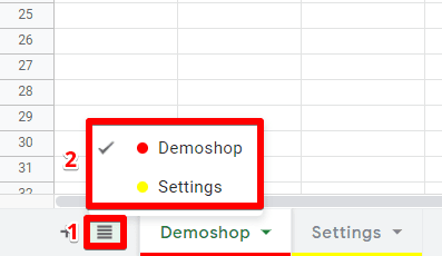
You can create multiple sheets in one Google Sheets file. Individual sheets are represented as tabs across the bottom of your screen. You can add sheets by clicking the plus sign ( + ), or see a list of all sheets by clicking the list button.

To rename a sheet, simply double-click on it and type a new name.

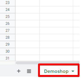
You can also add colors to a sheet by right-clicking the sheet tab (or clicking the menu arrow on the tab) and selecting Change color.

Then, you can select any color swatch to help highlight the sheet tab at the bottom of your screen.

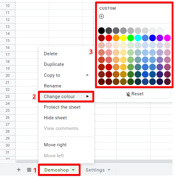
Note that this doesn’t affect any of the cell colors in the spreadsheet. This just helps you quickly navigate and identify sheets, or group related sheets by color.

Navigate and Organize Data with Columns and Rows

Each sheet is just a grid of cells organized by columns and rows. Columns are labeled alphabetically, and rows are labeled numerically.

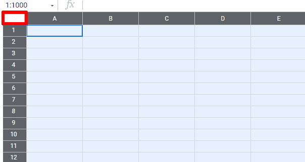
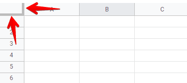
You can select data from multiple cells at a time if you want to apply an action to all of them. For example, to select the entire sheet, click the empty block between the column and row labels in the top left corner.

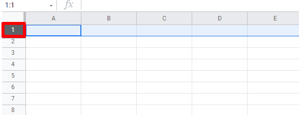
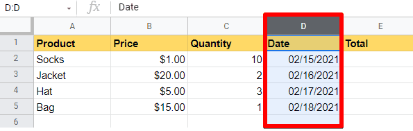
To select a whole column or row, click on its index letter or number.

You can freeze the first columns or rows by clicking and dragging the margin markers in the top left corner across the row or column that you want to freeze.

Freezing columns or rows allows them to always stay visible at any time, even if you scroll away from them across the spreadsheet. This is useful for column headers or row items that subsequent cells all describe.

In each cell, you can input data or calculations. Each cell is labeled with an index to identify it separately from the data it contains. The cell index is a combination of the indexes of columns and rows.

For example, the cell below is indexed as B2.

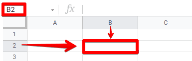
A cell’s index is important for formulas and functions, which can automatically make calculations with cell data, even if that data changes (since the index will remain the same) — more on this later.

Right-clicking the rows or columns will open quite a few options, many of which should be familiar (cut, copy, paste, etc.). However, some of these aren’t quite as self-explanatory, so we’ll demonstrate how they work.

Hiding a row or column doesn’t delete it. Instead, it will collapse the row or column and hide the cells until you click one of these arrows, which will expand it again.

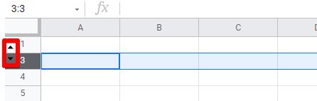
Hiding a row can be useful if you have lots of data that you need to keep but isn’t always relevant or useful. This can help you skip old data entries whenever you open the sheet if you only need to check newer data.

Grouping rows or columns can serve a similar purpose as the hiding option.

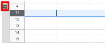
When you group several rows or columns, you can click on the minus ( – ) button to hide the entire group.

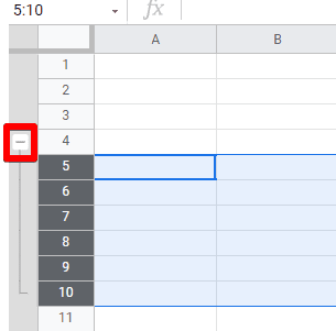
If the group is hidden, just click on the plus ( + ) button and they will re-appear.

You can always ungroup the rows or columns by selecting the group, right-clicking, and selecting the Ungroup option.

Create a Database with Google Sheets

The cells in your spreadsheet are good for all kinds of data, both quantitative and qualitative: dates, labels, prices, and more.

There are two ways of inputting data into an individual cell. Simply type into the cell directly, or select the cell and type in the function field (labeled fx).

The function field is especially useful when you want to use either long strings of text or formulas.

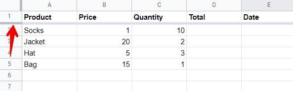
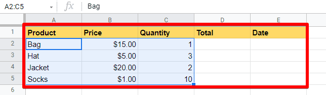
Let’s demonstrate with some basic data for a clothing store. (I find it helpful to bold the headers across the top of each column.)

You can freeze the first row by pulling the horizontal marker down from the top left corner. You’ll know that the row is frozen because of the bold marker in between the first and second rows.

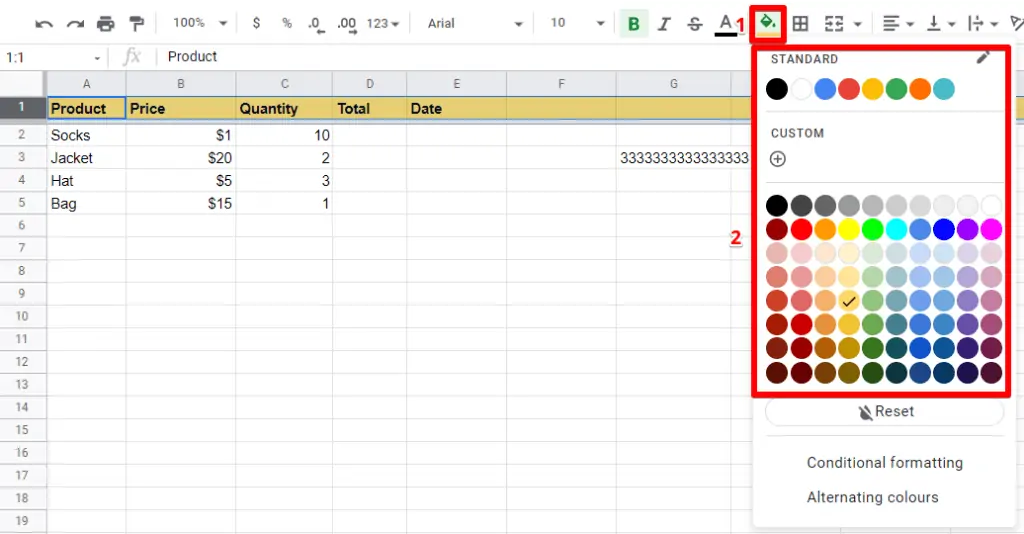
You can also add a background color to cells. This doesn’t affect the data at all, but colors can be visually helpful when reading data.

To add a background color, click on the Fill Color button and select a color to paint the selected cells. (Remember, you can select a whole row or column by clicking on its alphanumeric label.)

Some Useful Shortcuts, Navigation, and Selection Hotkeys

Wanna go fast? Here are some of the most common and useful shortcuts in Google Sheets:

For Mac:

Copy → ⌘ + C
Paste → ⌘ + V
Cut → ⌘ + X
Undo → ⌘ + Z
Redo →⌘ + Shift + Z
Directionally select all cells with value inputs → ⌘ + Shift + (direction arrow)
(For above, tap the directional arrow again to continue across the whole row or column.)
Select multiple cells → ⌘ + click
Select range of cells → Shift + click
Autofill cells → Click + drag corner of the cell
(For above, string data will copy the same string and simply paste it. Formulas will be transposed, and sequential data like dates will continue in order from the starting cell.)

For Windows:

Copy → Ctrl + C
Paste → Ctrl + V
Cut → Ctrl + X
Undo → Ctrl + Z
Redo → Ctrl + Shift + Z
Directionally select all cells with value inputs → Ctrl + Shift + (direction arrow)
(For above, tap the directional arrow again to continue across the whole row or column.)
Select multiple cells → Ctrl + click
Select range of cells → Shift + click
Autofill cells → Click + drag corner of the cell
(For above, string data will copy the same string and simply paste it. Formulas will be transposed, and sequential data like dates will continue in order from the starting cell.)

Note that if you copy more than one cell, those cells will keep their formatting when pasted. (More on this in the Special Paste Functions section of this guide.)

As you can see, it has the same structure and format. 

If you want to paste as plain text, you can use ⌘ / Ctrl + Shift + V.

🚨 Note: You can view the full list of keyboard shortcuts in Google Sheets by pressing ⌘ / Ctrl + /.

Format Data and Cells

You can adjust the data formatting of selected cells by using the Format menu. This is useful if you want to consistently present a column as currency or date, or if you want to apply dynamic colors or font effects. 

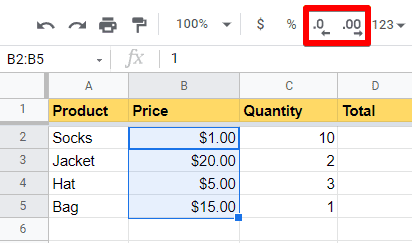
For example, let’s say that in this clothing shop’s database we want to format all prices to display as dollar values. Under Format → Number, select the Currency option to display the value in dollars and cents.

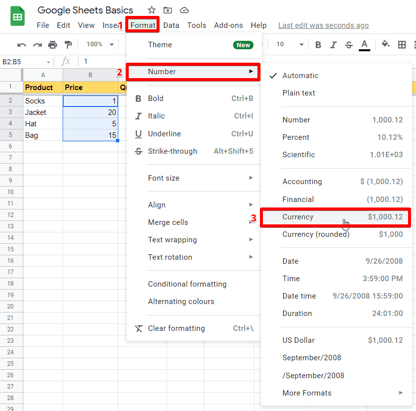
Note that you can also increase or decrease the number of decimal places in the menu bar. However, for currency, you’ll probably want to leave this at its default.

Basic Organization Features in Google Sheets

Text Wrapping

In some situations, your data entries are so large that they don’t fit inside individual cells.

Sometimes you’ll just expand your column width to accommodate this, but sometimes you’ll want to keep narrower columns. In this case, you have a couple of options to make your data easier to use depending on your situation.

Click on the Text Wrapping button to choose from one of the three following options: Overflow; Wrap; and Clip.

Overflow is pictured above, where the data string will continue past the column border into adjacent empty columns (until it runs into a column that contains data, where it will stop).

Wrap will expand the cell vertically to accommodate the data string. In other words, it will respect the column borders and continue the data string on a new line, making the entire row taller.

Finally, Clip will simply stop the data string when it reaches the column borders. The full data still exists and will be viewable when clicked in the function field, but it will not be visible on overview.

💡 Top Tip: Double-clicking the right side of the column will make it extend or shrink it to match the size of values from that column.

Special Paste Functions

As mentioned before, Google Sheets will copy both data fields and formatting by default.

But sometimes, you want to copy only certain aspects of your spreadsheet. You have a variety of options under Paste special.

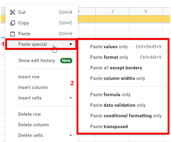
As you can see, there are different ways of pasting. Some of these are relatively self explanatory. Paste values only will paste only the displayed value from the copied cell, regardless of any functions or formulas used in the copied cell.

Paste format only will paste only the formatting rules without the data, while Paste all except borders pastes, data, and all formatting that excludes cell borders (which can include line widths and colors). Finally, Paste column widths only is useful for making the grid more spatially uniform.

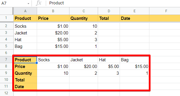
However, some of these paste functions are less intuitive. For example, Paste transposed will switch the columns and rows of the data.

Organize and Merge Cells

You can rearrange entire rows and columns that are already populated with data.

If you click on a row or column’s alphanumeric label and drag it up/down or left/right, it will move all of the cells and keep any formulas in order.

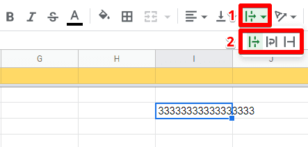
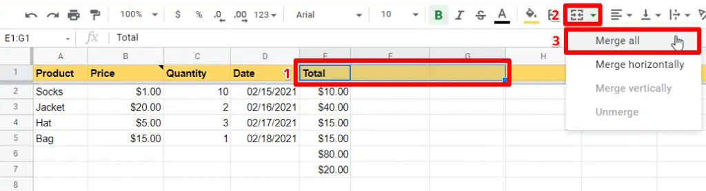
Sometimes you will want to have multiple columns under a single heading, or otherwise merge certain cells. You can do this by selecting any cells that you want to merge, then clicking the Merge icon.

You can select whether you want to merge a whole block of cells both vertically and horizontally, or choose a group of cells to merge only by row or column.

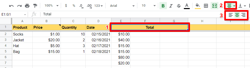
Once the cells have been merged, you’ll notice that there are no more lines between them. The data is shared in that cell between rows or columns.

Google Sheets aligns numbers on the right and text on the left on its own, but you can change the alignment of the cells if you’d like.

Sort and Organize Data by Values

To analyze or summarize your data, it’s useful to be able to see it sorted by the actual data values. For example, you might want it in chronological order, or descending price order, or alphabetical order.

To do this, select the column by which you would like to sort. Then, under the Data menu, you can choose to sort either ascending or descending, and either the whole sheet or just the selected range.

So what’s the difference?

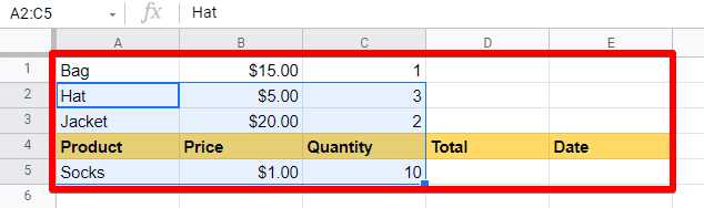
In the example below, the sheet below was sorted alphabetically by column A. This pulled the header down into the data (although you can avoid this by freezing the top row). Sorting the whole sheet is useful when you want all of your data organized in a particular way.

If you only want to sort part of your data, then you can Sort range instead of Sort sheet. This will sort only your selected range, which is useful if you have subheadings throughout your sheet for groups of related items.

Calculations and Data Analysis in Google Sheets

Basic Math Operations

In Google Sheets, you can use all regular math operators in the function field: addition + , subtraction – , multiplication * , and division / .

These math operations will update the value of a cell automatically if the data in related cells changes, which makes them great for automating data like revenue totals.

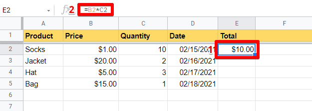
To demonstrate, let’s calculate the total revenue for each product at our sample clothing store by multiplying each product’s price with the quantity sold. 

Click on the cell that will contain your calculated data. Start all formulas with an equals sign ( = ). Then, you can either click on a cell or type its index to add it to the formula.

In this case, we want the final formula to read =B2*C2, using a star ( * ) as the multiplication operator. This will multiply the value in cell B2 by the value in cell C2, displaying the product in our selected formula cell E2.

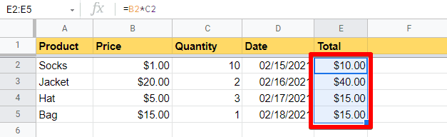
Easy, right? It gets better — simply click and drag the bottom right corner of the cell down to transpose the formula over other cells.

This means that the formula in cell E3 will read =B3*C3, the formula in cell E4 will be =B4*C4, and so on.

💡 Top Tip: Don’t want to transpose part of the formula? Add a dollar sign ( $ ) before the column index, row index, or both to freeze that index value. For example, the formula =F2*$G$2 would transpose the F2 index when pasted to another cell, but not the G2 index.

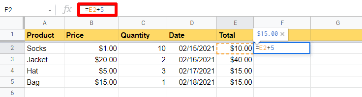
You can combine numerical values with cell indices in your calculations.

Let’s say that you want to add a shipping cost to each order of products in a separate column. You can select the cell index for the product order total (E2) and add it to a numeric value.

In the example below, the formula for cell F2 reads =E2+5.

Use Functions to Analyze Data

The best part about Google Sheets (and most other digital spreadsheets) is that you can automate calculations. Like your basic math operators, these calculations will update dynamically when you add or change data.

Some of the most commonly useful functions include SUM, AVERAGE, COUNT, MAX, and MIN. Once you understand how these work, you should be able to figure out how to use other functions, too.

To add one of these functions to a cell, select it and click the Functions icon — let’s start with SUM. 

Next, select all the cells that you want included in your calculation. If you want to sum cells E2, E3, E4, and E5, then simply click and drag over those four cells. This will add the function =SUM(E2:E5) to the function field.

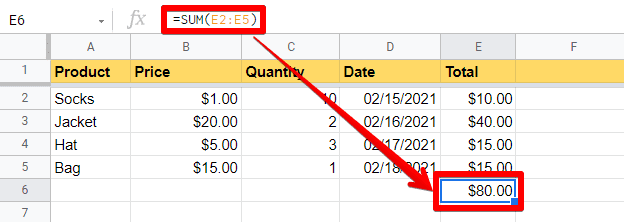
Whenever you click on the cell, the function field will display the formula, not the computed value. But in the spreadsheet overview, you’ll always see the calculated value — in this case, the sum of the prices in the cells above.

💡 Top Tip: Once you understand spreadsheet functions, you can also manually type the formulas into the function field to get the same result. Useful if you’re including lots of data!

Let’s try using the AVERAGE function for the same cells. You can select AVERAGE from the Functions menu, or you can simply type =AVERAGE(E2:E5).

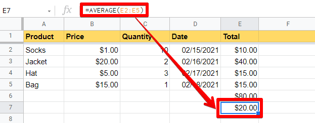
The process is essentially the same for all functions — start with an equal sign and the function name, then simply use a colon to denote the range between two cells (and remember to include parentheses around the range).

💡 Top Tip: Want to use an entire column in your calculation? Use just the column index on either side of the colon. For example, to sum all values in column A, use the formula =SUM(A:A)

Use Comments and Notes to Work with Your Team

Google Sheets is great for collaborating with other team members. Multiple people can edit one sheet at the same time, and you can leave comments for someone who will be working on the document later on using notes and comments.

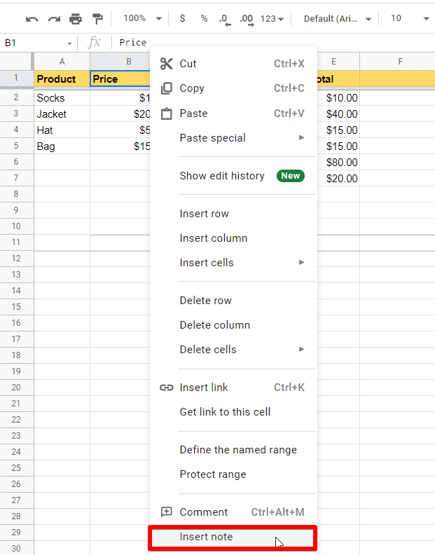
To insert a note, right-click a cell and select Insert Note.

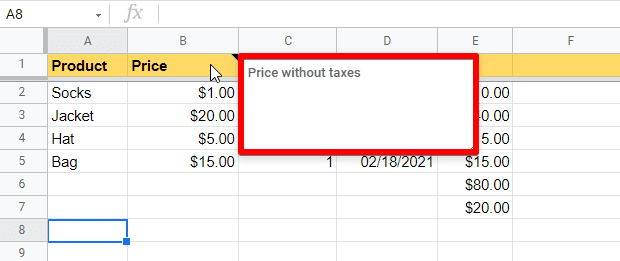
A small pop-up will open and there you can write your note, which can provide additional detail or context for data.

You’ll know that a cell has a note attached to it by the small black triangle that appears in the upper right corner. If you hover over that cell, the note will appear.

For less permanent messages to collaborators (i.e. issues to be checked or resolved), you should use comments instead of notes.

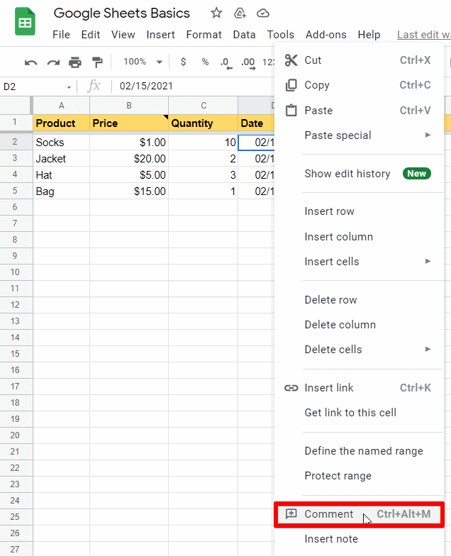
To insert a comment, right-click a cell and select Comment. (You can also use the shortcut ⌘ / Ctrl + Alt + M.)

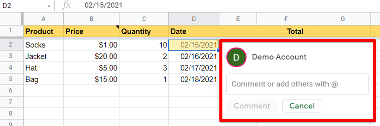
After that, Sheets will give you a popup on which you can type your comment. You can also tag someone using @ before their account name to send them an email notification about your comment.

Download or Export Google Spreadsheets

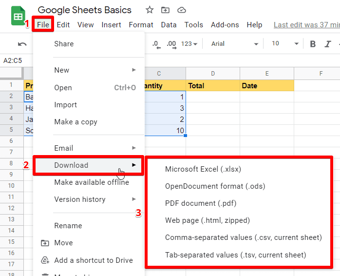
If you use other software to process data or want a PDF version of your spreadsheet, you can download in other formats.

Under File, select Download and choose your desired format. Your browser will do the rest and present you with a file in your selected file type. Easy!

Share Google Spreadsheets

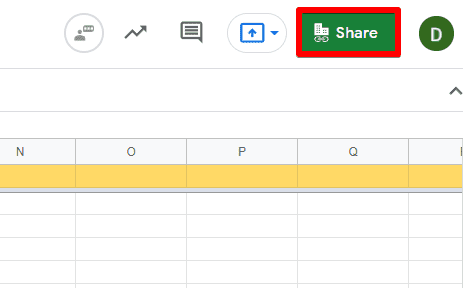
Sharing your spreadsheet with others in Google Sheets is easy — just click Share in the top right corner of your window.

Here, you can customize the type of access that specific Google accounts have to this spreadsheet. You can give individual accounts access to either View, Comment, or Edit.

You can also generate a special link to share your spreadsheet more universally. Click on Change to change the authorization for people entering via your share link.

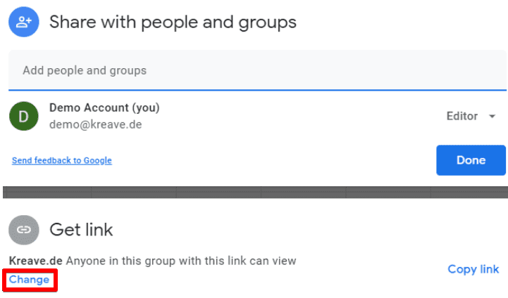
If you have a Google Workspace (formerly G Suite) domain, you will also have the option to specify sharing permissions for other users inside your group.

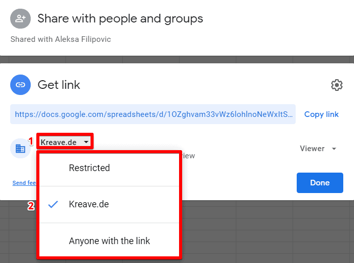
When you click on your group name, you can choose to give access to only specifically added accounts, any accounts inside your group, or anyone with the link.

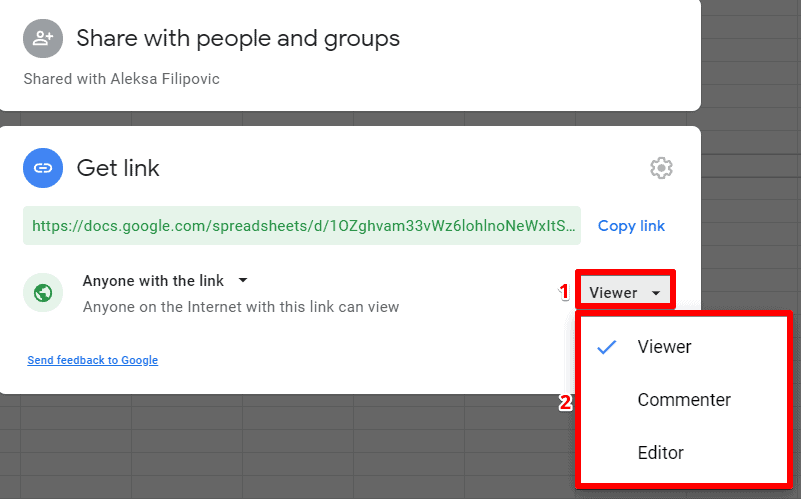
Then, you can select the level of authorization for accounts accessing this spreadsheet via your selected method. You can give Viewer, Commenter, or Editor permissions.

FAQ

Summary

And that covers most of the Google Sheets basics. You should be able to do all basic math operations and use Google Sheets functions to set up basic spreadsheets to support your work using these tips.

For more advanced features of Google Sheets, check out our handy guide on Data Analysis with Google Sheets.

What feature of Google Sheets have you found to be the most interesting? Are you using Comments and Notes to collaborate with your team members as well? Let us know in the comments below!

Subscribe & Get our FREE GTM for Beginners Course...

GET THE FREE COURSE